Дополнили линейку тарифов "СИЛА ДОМА" годовым тарифом. Принимаем заявки на подключение
Отличные новости! Подключиться выгодно по акции можно теперь до конца апреля
Сильный Интернет для Вашего Дома по выгодной цене! Принимаем заявки на подключение
Новый сезон тарифов объявляем открытым! :-)
Выбирай своё по духу, заряжайся позитивом - будь с Марком!
Будь как.......
Цены на оборудование беспрецедентно СНИЖЕНЫ!
Лови момент - подключай и наблюдай выгодно ;)
Принимаем заявки новоселов ЖК Оазис, Санвилл-1 и Санвилл-2 на подключение ко всем нашим цифровым услугам
Принимаем заявки жителей дома по адресу К. Маркса, 304а на подключение наших цифровых услуг
Новостройка по адресу Горького 157 уже в нашей сети. Принимаем заявки Новоселов на подключение Интернета и других цифровых услуг
Выгодный Интернет и Пакеты услуг для новых абонентов. Лосю не жалко - фиксирует цену на полгода!
Рады сообщить, что Новостройки ЖК Настроение-6, ЖК Ежевика-7 и ЖК Калинка парк-2 подключены к нашей сети! Принимаем заявки на подключение цифровых услуг
Новостройка по адресу 10 лет Октября 64а к2 подключена к нашей сети! Принимаем заявки жителей дома на подключение цифровых услуг
Обновленная версия мобильного приложения "Мой Марк" уже доступна для скачивания на Андроид.
Новостройка по адресу ул. 10 лет Октября, 64а корпус 1 уже с нашим Интернетом! Принимаем заявки новоселов
Продолжаем строить линию и подключать пригород Ижевска к скоростному Интернету и другим цифровым услугам
Ознакомьтесь с информацией об изменениях стоимости услуги по доставке документов для юр.лиц.
Новостройка по адресу ул. Васнецова, 38 в нашей сети. Принимаем заявки на подключение
Внимательно ознакомьтесь с информацией о способах оплаты!
Принимаем заявки на подключение интернета и других цифровых услуг в новостройке по адресу ул. Ухтомского, 11
Ознакомьтесь с информацией об услуге Др. Веб
Принимаем заявки на подключение интернета и других цифровых услуг в новостройке по адресу ул. Ипподромная, 17
350+ тв-каналов бесплатно до конца января
Поздравляем всех с Новым 2024 Годом и Рождеством!
Пожалуйста, ознакомьтесь с информацией о составе тарифов.
мы продолжаем череду подарков для наших абонентов беспроигрышной игрой – крути марковский Глюкофон и выигрывай!
Игра завершена!
В сети нашего КТВ появились 2 новых канала